Interpretable Modelling of Credit Risk
As detailed in Cynthia Rudin’s excellent commentary on interpretability (ArXiV version here), there are a plethora of reasons to avoid the use of black box models when models are being used to make high stakes decisions to may have life-altering effects on real people. Efforts to develop “explainable black box models,” while appealing for their potential to let us continuing using the same tools we always have and to creation explanations after the fact, are inherently flawed. As Rudin notes in my single favorite passage from her paper:
Explainable ML methods provide explanations that are not faithful to what the original model computes. Explanations must be wrong. They cannot have perfect fidelity with respect to the original model. If the explanation was completely faithful to what the original model computes, the explanation would equal the original model, and one would not need the original model in the first place, only the explanation. (In other words, this is a case where the original model would be interpretable.) This leads to the danger that any explanation method for a black box model can be an inaccurate representation of the original model in parts of the feature space.
An inaccurate (low-fidelity) explanation model limits trust in the explanation, and by extension, trust in the black box that it is trying to explain. An explainable model that has a 90% agreement with the original model indeed explains the original model most of the time. However, an explanation model that is correct 90% of the time is wrong 10% of the time. If a tenth of the explanations are incorrect, one cannot trust the explanations, and thus one cannot trust the original black box. If we cannot know for certain whether our explanation is correct, we cannot know whether to trust either the explanation or the original model.
With this motivation in mind, in this exercise, we will use a cutting edge interpretable modeling framework to model credit risk using data from the 14th Pacific-Asia Knowledge Discovery and Data Mining conference (PAKDD 2010). This data covers the period of 2006 to 2009, and “comes from a private label credit card operation of a Brazilian credit company and its partner shops.” (The competition was won by TIMi, who purely by coincidence helped me complete my PhD dissertation research!).
We will be working with Generalized Additive Models (GAMs) (not to be confused with Generalized Linear Models (GLMs) — GLMs are a special case of GAMs). In particular, we will be using the pyGAM, though this is far from the only GAM implementation out there. mvgam in R is probably considered the gold standard, as it was developed by a pioneering researcher of GAMs. statsmodels also has an implementation, and GAM is also hiding in plain sight behind many other tools, like Meta’s Prophet time series forecasting library (which is GAM-based).
WARNING: Mis-specified or poorly specified pyGAM models can take forever (hours, days, etc.) to estimate. Nothing in this exercise should take more than, at most a few minutes to estimate even on a commodity laptop. If you find your model is taking longer than that to run, stop and check your specification. Categorical variables with tons of unique values, in particular, can make numerical optimization very difficult.
Data Prep
Exercise 1
The PADD 2010 data is in this repository. You can find column names in PAKDD2010_VariablesList.XLS and the actual data in PAKDD2010_Modeling_Data.txt.
Note: you may run into a string-encoding issue loading the PAKDD2010_Modeling_Data.txt data. All I’ll say is that most latin-based languages used latin8 as a text encoding prior to broad adoption of UTF-8. (Don’t know about UTF? Check out this video!)
Load the data (including column names).
[1]:
import pandas as pd
import numpy as np

pd.set_option("mode.copy_on_write", True)
pd.set_option(
    "display.max_columns", 999
)  # Not the cleanest trick, but ok from time to time.
[2]:
# read in column variables
column_names = pd.read_excel(
    "https://github.com/nickeubank/MIDS_Data/raw/"
    "master/PAKDD%202010/PAKDD2010_VariablesList.XLS"
)
column_names.loc[column_names["Var_Title"].duplicated(), "Var_Title"] += "_02"

assert not column_names["Var_Title"].duplicated().any()
columnlist = column_names["Var_Title"].tolist()
[3]:
apps = pd.read_csv(
    "https://github.com/nickeubank/MIDS_Data/raw/"
    "master/PAKDD%202010/PAKDD2010_Modeling_Data.txt",
    sep="\t",
    names=columnlist,
    na_values=["NULL", "", " "],
    encoding="latin8",
)
apps.head()
/var/folders/fs/h_8_rwsn5hvg9mhp0txgc_s9v6191b/T/ipykernel_42350/3209276034.py:1: DtypeWarning: Columns (51,52) have mixed types. Specify dtype option on import or set low_memory=False.
  apps = pd.read_csv(
[3]:
| ID_CLIENT | CLERK_TYPE | PAYMENT_DAY | APPLICATION_SUBMISSION_TYPE | QUANT_ADDITIONAL_CARDS | POSTAL_ADDRESS_TYPE | SEX | MARITAL_STATUS | QUANT_DEPENDANTS | EDUCATION_LEVEL | STATE_OF_BIRTH | CITY_OF_BIRTH | NACIONALITY | RESIDENCIAL_STATE | RESIDENCIAL_CITY | RESIDENCIAL_BOROUGH | FLAG_RESIDENCIAL_PHONE | RESIDENCIAL_PHONE_AREA_CODE | RESIDENCE_TYPE | MONTHS_IN_RESIDENCE | FLAG_MOBILE_PHONE | FLAG_EMAIL | PERSONAL_MONTHLY_INCOME | OTHER_INCOMES | FLAG_VISA | FLAG_MASTERCARD | FLAG_DINERS | FLAG_AMERICAN_EXPRESS | FLAG_OTHER_CARDS | QUANT_BANKING_ACCOUNTS | QUANT_SPECIAL_BANKING_ACCOUNTS | PERSONAL_ASSETS_VALUE | QUANT_CARS | COMPANY | PROFESSIONAL_STATE | PROFESSIONAL_CITY | PROFESSIONAL_BOROUGH | FLAG_PROFESSIONAL_PHONE | PROFESSIONAL_PHONE_AREA_CODE | MONTHS_IN_THE_JOB | PROFESSION_CODE | OCCUPATION_TYPE | MATE_PROFESSION_CODE | EDUCATION_LEVEL_02 | FLAG_HOME_ADDRESS_DOCUMENT | FLAG_RG | FLAG_CPF | FLAG_INCOME_PROOF | PRODUCT | FLAG_ACSP_RECORD | AGE | RESIDENCIAL_ZIP_3 | PROFESSIONAL_ZIP_3 | TARGET_LABEL_BAD=1 | |
|---|---|---|---|---|---|---|---|---|---|---|---|---|---|---|---|---|---|---|---|---|---|---|---|---|---|---|---|---|---|---|---|---|---|---|---|---|---|---|---|---|---|---|---|---|---|---|---|---|---|---|---|---|---|---|
| 0 | 1 | C | 5 | Web | 0 | 1 | F | 6 | 1 | 0 | RN | Assu | 1 | RN | Santana do Matos | Centro | Y | 105.0 | 1.0 | 15.0 | N | 1 | 900.0 | 0.0 | 1 | 1 | 0 | 0 | 0 | 0 | 0 | 0.0 | 0 | N | NaN | NaN | NaN | N | NaN | 0 | 9.0 | 4.0 | NaN | NaN | 0 | 0 | 0 | 0 | 1 | N | 32 | 595 | 595 | 1 |
| 1 | 2 | C | 15 | Carga | 0 | 1 | F | 2 | 0 | 0 | RJ | rio de janeiro | 1 | RJ | RIO DE JANEIRO | CAMPO GRANDE | Y | 20.0 | 1.0 | 1.0 | N | 1 | 750.0 | 0.0 | 0 | 0 | 0 | 0 | 0 | 0 | 0 | 0.0 | 0 | Y | NaN | NaN | NaN | N | NaN | 0 | 11.0 | 4.0 | 11.0 | NaN | 0 | 0 | 0 | 0 | 1 | N | 34 | 230 | 230 | 1 |
| 2 | 3 | C | 5 | Web | 0 | 1 | F | 2 | 0 | 0 | RN | GARANHUNS | 1 | RN | Parnamirim | Boa Esperanca | Y | 105.0 | 1.0 | NaN | N | 1 | 500.0 | 0.0 | 0 | 0 | 0 | 0 | 0 | 0 | 0 | 0.0 | 0 | N | NaN | NaN | NaN | N | NaN | 0 | 11.0 | NaN | NaN | NaN | 0 | 0 | 0 | 0 | 1 | N | 27 | 591 | 591 | 0 |
| 3 | 4 | C | 20 | Web | 0 | 1 | F | 2 | 0 | 0 | PE | CABO | 1 | PE | CABO | PONTE DOS CARVALHOS | N | NaN | NaN | NaN | N | 1 | 500.0 | 0.0 | 0 | 0 | 0 | 0 | 0 | 0 | 0 | 0.0 | 0 | N | NaN | NaN | NaN | N | NaN | 0 | NaN | NaN | NaN | NaN | 0 | 0 | 0 | 0 | 1 | N | 61 | 545 | 545 | 0 |
| 4 | 5 | C | 10 | Web | 0 | 1 | M | 2 | 0 | 0 | RJ | RIO DE JANEIRO | 1 | RJ | Rio de Janeiro | Santa Cruz | Y | 20.0 | 1.0 | 12.0 | N | 1 | 1200.0 | 0.0 | 0 | 0 | 0 | 0 | 0 | 0 | 0 | 0.0 | 0 | N | NaN | NaN | NaN | N | NaN | 0 | 9.0 | 5.0 | NaN | NaN | 0 | 0 | 0 | 0 | 1 | N | 48 | 235 | 235 | 1 |
[4]:
apps.describe()
[4]:
| ID_CLIENT | PAYMENT_DAY | QUANT_ADDITIONAL_CARDS | POSTAL_ADDRESS_TYPE | MARITAL_STATUS | QUANT_DEPENDANTS | EDUCATION_LEVEL | NACIONALITY | RESIDENCIAL_PHONE_AREA_CODE | RESIDENCE_TYPE | MONTHS_IN_RESIDENCE | FLAG_EMAIL | PERSONAL_MONTHLY_INCOME | OTHER_INCOMES | FLAG_VISA | FLAG_MASTERCARD | FLAG_DINERS | FLAG_AMERICAN_EXPRESS | FLAG_OTHER_CARDS | QUANT_BANKING_ACCOUNTS | QUANT_SPECIAL_BANKING_ACCOUNTS | PERSONAL_ASSETS_VALUE | QUANT_CARS | PROFESSIONAL_PHONE_AREA_CODE | MONTHS_IN_THE_JOB | PROFESSION_CODE | OCCUPATION_TYPE | MATE_PROFESSION_CODE | EDUCATION_LEVEL_02 | FLAG_HOME_ADDRESS_DOCUMENT | FLAG_RG | FLAG_CPF | FLAG_INCOME_PROOF | PRODUCT | AGE | TARGET_LABEL_BAD=1 | |
|---|---|---|---|---|---|---|---|---|---|---|---|---|---|---|---|---|---|---|---|---|---|---|---|---|---|---|---|---|---|---|---|---|---|---|---|---|
| count | 50000.000000 | 50000.000000 | 50000.0 | 50000.000000 | 50000.00000 | 50000.000000 | 50000.0 | 50000.000000 | 41788.000000 | 48651.000000 | 46223.000000 | 50000.000000 | 50000.000000 | 50000.000000 | 50000.000000 | 50000.000000 | 50000.000000 | 50000.000000 | 50000.000000 | 50000.000000 | 50000.000000 | 5.000000e+04 | 50000.000000 | 13468.000000 | 50000.000000 | 42244.000000 | 42687.000000 | 21116.000000 | 17662.000000 | 50000.0 | 50000.0 | 50000.0 | 50000.0 | 50000.000000 | 50000.00000 | 50000.000000 |
| mean | 25000.500000 | 12.869920 | 0.0 | 1.006540 | 2.14840 | 0.650520 | 0.0 | 0.961600 | 64.544223 | 1.252225 | 9.727149 | 0.802280 | 886.678437 | 35.434760 | 0.111440 | 0.097460 | 0.001320 | 0.001740 | 0.002040 | 0.357840 | 0.357840 | 2.322372e+03 | 0.336140 | 62.397015 | 0.009320 | 8.061784 | 2.484316 | 3.797926 | 0.296003 | 0.0 | 0.0 | 0.0 | 0.0 | 1.275700 | 43.24852 | 0.260820 |
| std | 14433.901067 | 6.608385 | 0.0 | 0.080606 | 1.32285 | 1.193655 | 0.0 | 0.202105 | 38.511833 | 0.867833 | 10.668841 | 0.398284 | 7846.959327 | 891.515142 | 0.314679 | 0.296586 | 0.036308 | 0.041677 | 0.045121 | 0.479953 | 0.479953 | 4.235798e+04 | 0.472392 | 36.622626 | 0.383453 | 3.220104 | 1.532261 | 5.212168 | 0.955688 | 0.0 | 0.0 | 0.0 | 0.0 | 0.988286 | 14.98905 | 0.439086 |
| min | 1.000000 | 1.000000 | 0.0 | 1.000000 | 0.00000 | 0.000000 | 0.0 | 0.000000 | 1.000000 | 0.000000 | 0.000000 | 0.000000 | 60.000000 | 0.000000 | 0.000000 | 0.000000 | 0.000000 | 0.000000 | 0.000000 | 0.000000 | 0.000000 | 0.000000e+00 | 0.000000 | 1.000000 | 0.000000 | 0.000000 | 0.000000 | 0.000000 | 0.000000 | 0.0 | 0.0 | 0.0 | 0.0 | 1.000000 | 6.00000 | 0.000000 |
| 25% | 12500.750000 | 10.000000 | 0.0 | 1.000000 | 1.00000 | 0.000000 | 0.0 | 1.000000 | 29.000000 | 1.000000 | 1.000000 | 1.000000 | 360.000000 | 0.000000 | 0.000000 | 0.000000 | 0.000000 | 0.000000 | 0.000000 | 0.000000 | 0.000000 | 0.000000e+00 | 0.000000 | 29.000000 | 0.000000 | 9.000000 | 1.000000 | 0.000000 | 0.000000 | 0.0 | 0.0 | 0.0 | 0.0 | 1.000000 | 31.00000 | 0.000000 |
| 50% | 25000.500000 | 10.000000 | 0.0 | 1.000000 | 2.00000 | 0.000000 | 0.0 | 1.000000 | 68.000000 | 1.000000 | 6.000000 | 1.000000 | 500.000000 | 0.000000 | 0.000000 | 0.000000 | 0.000000 | 0.000000 | 0.000000 | 0.000000 | 0.000000 | 0.000000e+00 | 0.000000 | 66.000000 | 0.000000 | 9.000000 | 2.000000 | 0.000000 | 0.000000 | 0.0 | 0.0 | 0.0 | 0.0 | 1.000000 | 41.00000 | 0.000000 |
| 75% | 37500.250000 | 15.000000 | 0.0 | 1.000000 | 2.00000 | 1.000000 | 0.0 | 1.000000 | 100.000000 | 1.000000 | 15.000000 | 1.000000 | 800.000000 | 0.000000 | 0.000000 | 0.000000 | 0.000000 | 0.000000 | 0.000000 | 1.000000 | 1.000000 | 0.000000e+00 | 1.000000 | 97.000000 | 0.000000 | 9.000000 | 4.000000 | 11.000000 | 0.000000 | 0.0 | 0.0 | 0.0 | 0.0 | 1.000000 | 53.00000 | 1.000000 |
| max | 50000.000000 | 25.000000 | 0.0 | 2.000000 | 7.00000 | 53.000000 | 0.0 | 2.000000 | 126.000000 | 5.000000 | 228.000000 | 1.000000 | 959000.000000 | 194344.000000 | 1.000000 | 1.000000 | 1.000000 | 1.000000 | 1.000000 | 2.000000 | 2.000000 | 6.000000e+06 | 1.000000 | 126.000000 | 35.000000 | 18.000000 | 5.000000 | 17.000000 | 5.000000 | 0.0 | 0.0 | 0.0 | 0.0 | 7.000000 | 106.00000 | 1.000000 |
[5]:
# The equal sign causes headaches
apps = apps.rename(columns={"TARGET_LABEL_BAD=1": "TARGET_LABEL_BAD_1"})
Exercise 2
There are a few variables with a lot of missing values (more than half missing). Given the limited documentation for this data it’s a little hard to be sure why, but given the effect on sample size and what variables are missing, let’s go ahead and drop them. You you end up dropping 6 variables.
Hint: Some variables have missing values that aren’t immediately obviously.
(This is not strictly necessary at this stage, given we’ll be doing more feature selection down the line, but keeps things easier knowing we don’t have to worry about missingness later.)
[6]:
# Note that this code only works because I modified the
# read_csv code above by adding `na_values=["NULL", "", " "]`.
# If you don't have that, this code will not drop the columns in question.
to_drop = [c for c in apps.columns if apps[c].isnull().mean() > 0.5]
to_drop
[6]:
['PROFESSIONAL_STATE',
 'PROFESSIONAL_CITY',
 'PROFESSIONAL_BOROUGH',
 'PROFESSIONAL_PHONE_AREA_CODE',
 'MATE_PROFESSION_CODE',
 'EDUCATION_LEVEL_02']
[7]:
apps = apps.drop(columns=to_drop)
Exercise 3
Next up, we’re going to fit a GAM model on this data. Before we do so below, however, we need to make sure we’re comfortable with the features we’re using.
"QUANT_DEPENDANTS",
"QUANT_CARS",
"MONTHS_IN_RESIDENCE",
"PERSONAL_MONTHLY_INCOME",
"QUANT_BANKING_ACCOUNTS",
"AGE",
"SEX",
"MARITAL_STATUS",
"OCCUPATION_TYPE",
"RESIDENCE_TYPE",
"RESIDENCIAL_STATE",
"RESIDENCIAL_CITY",
"RESIDENCIAL_BOROUGH",
"RESIDENCIAL_ZIP_3"
(GAMs don’t have any automatic feature selection methods, so these are based on my own sense of features that are likely to matter. A fully analysis would entail a few passes at feature refinement)
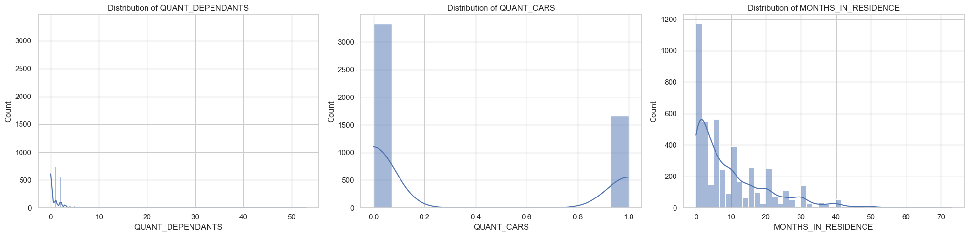
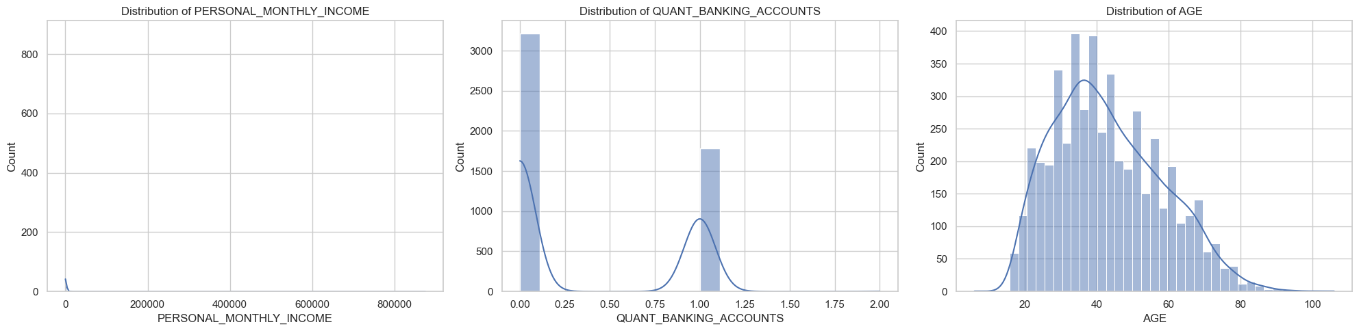
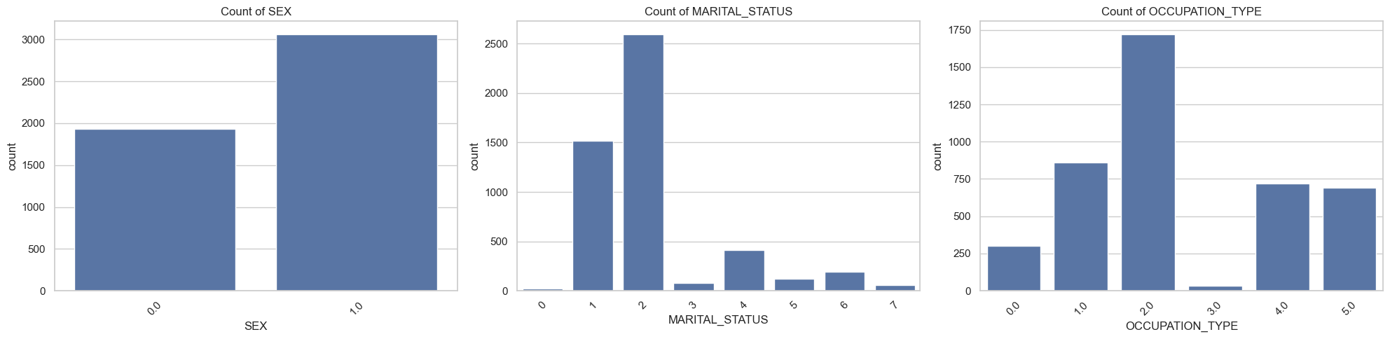
Plot and otherwise characterize the distributions of all the variables we may use. If you see anything bananas, adjust how terms enter your model. Yes, pyGAM has flexible functional forms, but giving the model features that are engineered to be more substantively meaningful (e.g., taking log of income) will aid model estimation.
You should probably do something about the functional form of at least PERSONAL_MONTHLY_INCOME, and QUANT_DEPENDANTS.
[8]:
numeric_columns = [
    "QUANT_DEPENDANTS",
    "QUANT_CARS",
    "MONTHS_IN_RESIDENCE",
    "PERSONAL_MONTHLY_INCOME",
    "QUANT_BANKING_ACCOUNTS",
    "AGE",
]
cat_columns = [
    "SEX",
    "MARITAL_STATUS",
    "OCCUPATION_TYPE",
    "RESIDENCE_TYPE",
    "RESIDENCIAL_PHONE_AREA_CODE",
    "RESIDENCIAL_ZIP_3",
    "RESIDENCIAL_STATE",
    "RESIDENCIAL_CITY",
    "RESIDENCIAL_BOROUGH",
]
[9]:
print(
    f"{len(numeric_columns)} initially numeric, {len(cat_columns)} initially categorical"
)
6 initially numeric, 9 initially categorical
[10]:
# prompt: map M=1, F=2, to 'sex' value
apps["SEX"].value_counts()
apps["SEX"] = apps["SEX"].replace({"M": 0, "F": 1, "N": np.nan})
apps["SEX"].value_counts()
/var/folders/fs/h_8_rwsn5hvg9mhp0txgc_s9v6191b/T/ipykernel_42350/1606787409.py:3: FutureWarning: Downcasting behavior in `replace` is deprecated and will be removed in a future version. To retain the old behavior, explicitly call `result.infer_objects(copy=False)`. To opt-in to the future behavior, set `pd.set_option('future.no_silent_downcasting', True)`
  apps["SEX"] = apps["SEX"].replace({"M": 0, "F": 1, "N": np.nan})
[10]:
SEX
1.0    30805
0.0    19130
Name: count, dtype: int64
[11]:
for col in numeric_columns:
    apps[col] = pd.to_numeric(apps[col], errors="coerce")
[12]:
import seaborn as sns
import matplotlib.pyplot as plt
sns.set_theme(style="whitegrid")
apps_sampled = apps.sample(frac=0.1, random_state=42)
# Plotting Numeric Columns
for i, column in enumerate(numeric_columns):
if i % 3 == 0: # Start a new row for every 3 plots
plt.figure(figsize=(20, 5))
plt.subplot(1, 3, (i % 3) + 1)
sns.histplot(apps_sampled[column], kde=True)
plt.title(f"Distribution of {column}")
if (i % 3 == 2) or (i == len(numeric_columns) - 1):
plt.tight_layout()
plt.show()
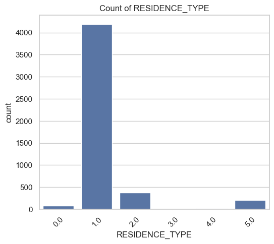
# Plotting Categorical Columns
for i, column in enumerate(cat_columns):
if apps[column].nunique() < 15:
if i % 3 == 0: # Start a new row for every 3 plots
plt.figure(figsize=(20, 5))
plt.subplot(1, 3, (i % 3) + 1)
sns.countplot(x=column, data=apps_sampled)
plt.title(f"Count of {column}")
plt.xticks(rotation=45)
if (i % 3 == 2) or (i == len(cat_columns) - 1):
plt.tight_layout()
plt.show()
[13]:
# Functional form tweaks for income and months in residence.
apps["PERSONAL_MONTHLY_INCOME"] = np.log(apps["PERSONAL_MONTHLY_INCOME"])

apps["MONTHS_IN_RESIDENCE"] = np.log(apps["MONTHS_IN_RESIDENCE"] + 1)

# For Dependents I'll pool some of the values into categories (three or more kids seems reasonable).
apps.loc[apps["QUANT_DEPENDANTS"] > 3, "QUANT_DEPENDANTS"] = 3
apps["QUANT_DEPENDANTS"] = apps["QUANT_DEPENDANTS"].astype("category")
apps["QUANT_DEPENDANTS"].value_counts()

# Collapse other marital categories
apps["MARITAL_STATUS"] = apps["MARITAL_STATUS"].astype("int")
apps.loc[apps["MARITAL_STATUS"] > 3, "MARITAL_STATUS"] = 3
Exercise 4
Geographic segregation means residency data often contains LOTS of information. But there’s a problem with RESIDENCIAL_CITY and RESIDENCIAL_BOROUGH. What is the problem?
In any real project, this would be something absolutely worth resolving, but for this exercise, we’ll just drop all three string RESIDENCIAL_ variables.
The strings are SUPER DIRTY, with lots of slightly different spellings of the same places. It can be fixed, but would take significant time.
Model Fitting
Exercise 5
First, use train_test_split to do an 80/20 split of your data. Then, using the TARGET_LABEL_BAD variable, fit a classification model on this data. Optimize with gridsearch. Use splines for continuous variables and factors for categoricals.
At this point we’d ideally be working with 11 variables. However pyGAM can get a little slow with factor features with lots of values + lots of unique values (e.g., 50,000 observations and the many values of RESIDENCIAL_ZIP takes about 15 minutes on my computer). In that configuration, you should get a model fit in 10-15 seconds.
So let’s start by fitting a model that also excludes RESIDENCIAL_ZIP.
[14]:
numeric_columns = [
    "PERSONAL_MONTHLY_INCOME",
    "AGE",
    "MONTHS_IN_RESIDENCE",
]

cat_columns = [
    "QUANT_DEPENDANTS",
    "SEX",
    "QUANT_CARS",
    "MARITAL_STATUS",
    "OCCUPATION_TYPE",
    "RESIDENCE_TYPE",
    "QUANT_BANKING_ACCOUNTS",
]
[15]:
print(
    f"{len(numeric_columns)} initially numeric, {len(cat_columns)} initially categorical"
)
3 initially numeric, 7 initially categorical
[16]:
X = apps[numeric_columns + cat_columns + ["TARGET_LABEL_BAD_1"]]
X["QUANT_DEPENDANTS"] = X["QUANT_DEPENDANTS"].cat.codes
# X["RESIDENCIAL_ZIP_3"] = pd.to_numeric(X["RESIDENCIAL_ZIP_3"], errors="coerce")
X = X.dropna()
y = X["TARGET_LABEL_BAD_1"].copy()
X = X.drop(columns="TARGET_LABEL_BAD_1")
print(f"Dropping missing gives sample size of {len(X):,.0f} (from 50,000 possible)")
Dropping missing gives sample size of 40,400 (from 50,000 possible)
[17]:
X["SEX"] = X["SEX"].astype("int")
[18]:
from sklearn.model_selection import train_test_split

X_train, X_test, y_train, y_test = train_test_split(
    X, y, test_size=0.2, random_state=42
)
[19]:
# This is helpful just to keep track of feature numbers. :)
from pygam import LogisticGAM, s, f

for i, c in enumerate(X.columns):
    print(f"{i}: {c}")
0: PERSONAL_MONTHLY_INCOME
1: AGE
2: MONTHS_IN_RESIDENCE
3: QUANT_DEPENDANTS
4: SEX
5: QUANT_CARS
6: MARITAL_STATUS
7: OCCUPATION_TYPE
8: RESIDENCE_TYPE
9: QUANT_BANKING_ACCOUNTS
[20]:
terms = s(0) + s(1) + s(2) + f(3) + f(4) + f(5) + f(6) + f(7) + f(8) + f(9)

gam = LogisticGAM(terms=terms)
gam.gridsearch(X_train.values, y_train.values)
  0% (0 of 11) |                         | Elapsed Time: 0:00:00 ETA:  --:--:--
  9% (1 of 11) |##                       | Elapsed Time: 0:00:01 ETA:   0:00:11
 18% (2 of 11) |####                     | Elapsed Time: 0:00:02 ETA:   0:00:09
 27% (3 of 11) |######                   | Elapsed Time: 0:00:03 ETA:   0:00:08
 36% (4 of 11) |#########                | Elapsed Time: 0:00:03 ETA:   0:00:06
 45% (5 of 11) |###########              | Elapsed Time: 0:00:04 ETA:   0:00:05
 54% (6 of 11) |#############            | Elapsed Time: 0:00:05 ETA:   0:00:04
 63% (7 of 11) |###############          | Elapsed Time: 0:00:06 ETA:   0:00:03
 72% (8 of 11) |##################       | Elapsed Time: 0:00:06 ETA:   0:00:02
 81% (9 of 11) |####################     | Elapsed Time: 0:00:07 ETA:   0:00:01
 90% (10 of 11) |#####################   | Elapsed Time: 0:00:08 ETA:   0:00:00
100% (11 of 11) |########################| Elapsed Time: 0:00:08 Time:  0:00:08
[20]:
LogisticGAM(callbacks=[Deviance(), Diffs(), Accuracy()],
   fit_intercept=True, max_iter=100,
   terms=s(0) + s(1) + s(2) + f(3) + f(4) + f(5) + f(6) + f(7) + f(8) + f(9) + intercept,
   tol=0.0001, verbose=False)
Exercise 6
Create a (naive) confusion matrix using the predicted values you get with predict() on your test data. Our stakeholder cares about two things:
maximizing the number of people to whom they extend credit, and
the false omission rate (the share of people identified as “safe bets” who aren’t, and who thus default).
How many “good bets” does the model predict (true negatives), and what is the False Omission Rate (the share of predicted negatives that are false negatives)?
Looking at the confusion matrix, how did the model maximize accuracy?
[21]:
confusion_matrix = pd.crosstab(
    y_test,
    gam.predict(X_test).astype("int"),
    rownames=["Actually Bad"],
    colnames=["Predicted Bad"],
)
true_negatives = confusion_matrix.loc[0, 0]
false_negatives = confusion_matrix.loc[1, 0]
false_omission_rate = false_negatives / (false_negatives + true_negatives)

print(f"Confusion Matrix: \n{confusion_matrix}")
print(f"Num true negatives is {true_negatives:,.0f}")
print(f"False omission rate for {false_omission_rate:.2%}")
Confusion Matrix:
Predicted Bad     0  1
Actually Bad
0              5978  0
1              2101  1
Num true negatives is 5,978
False omission rate for 26.01%
We have high accuracy because it just predicting “everyone’s ok!”. Because the data is pretty imbalanced, that worked! But not really what we want.
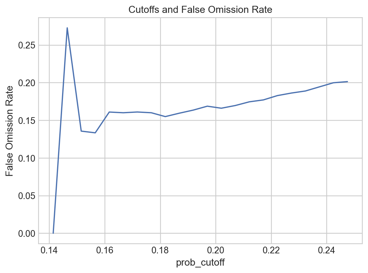
Exercise 7
Suppose your stakeholder wants to minimize the share of negative predictions that are false negatives. How low of a False Omission Rate can you get (assuming more than, say, 10 true negatives), and how many “good bets” (true negatives) do they get at that risk level?
Hint: use predict_proba()
Note: One can use class weights to shift the emphasis of the original model fitting, but for the moment let’s just play with predict_proba() and thresholds.
[22]:
#########
# I'm gonna do this in two ways.
# First, just kinda by print statement —
# not really ideal, but works.
#
# I'll do the more rigorous way below.
#########

for i in np.arange(0, 0.3, 0.025):
    confusion_matrix = pd.crosstab(
        y_test,
        (gam.predict_proba(X_test) > i).astype("int"),
        rownames=["Actually Bad"],
        colnames=["Predicted Bad"],
    )

    if (gam.predict_proba(X_test) > i).mean() != 1:
        true_negatives = confusion_matrix.loc[0, 0]
        false_negatives = confusion_matrix.loc[1, 0]
        false_omission_rate = false_negatives / (false_negatives + true_negatives)

    print(f"False Omission rate for {i:.3f} is {false_omission_rate:.2%}")
    print(f"Number of true negatives at {i:.2f} is {true_negatives:,.0f}")
    print()
False Omission rate for 0.000 is 26.01%
Number of true negatives at 0.00 is 5,978

False Omission rate for 0.025 is 26.01%
Number of true negatives at 0.03 is 5,978

False Omission rate for 0.050 is 26.01%
Number of true negatives at 0.05 is 5,978

False Omission rate for 0.075 is 26.01%
Number of true negatives at 0.08 is 5,978

False Omission rate for 0.100 is 26.01%
Number of true negatives at 0.10 is 5,978

False Omission rate for 0.125 is 26.01%
Number of true negatives at 0.12 is 5,978

False Omission rate for 0.150 is 15.91%
Number of true negatives at 0.15 is 37

False Omission rate for 0.175 is 15.89%
Number of true negatives at 0.18 is 434

False Omission rate for 0.200 is 16.75%
Number of true negatives at 0.20 is 1,183

False Omission rate for 0.225 is 18.60%
Number of true negatives at 0.23 is 1,995

False Omission rate for 0.250 is 20.39%
Number of true negatives at 0.25 is 2,882

False Omission rate for 0.275 is 21.82%
Number of true negatives at 0.28 is 3,838
If we use the cutpoint of
0.175, we have a False Omission Rate of ~16%, and 434 true negatives.
[23]:
###########
# The more rigorous way!
###########


def get_neg_stats(grid, model, X, y_true):
    negs = pd.DataFrame(
        zip(*map(lambda i: omission_rate(i, model.predict_proba(X), y_true), grid))
    ).T
    negs["prob_cutoff"] = grid
    negs = negs.rename(columns={0: "False Omission Rate", 1: "True Negatives"})
    return negs


def omission_rate(i, predicted, y_true):

    confusion_matrix = pd.crosstab(
        y_true,
        (predicted > i).astype("int"),
        rownames=["Actually Bad"],
        colnames=["Predicted Bad"],
    )

    if (predicted > i).mean() != 1:
        true_negatives = confusion_matrix.loc[0, 0]
        false_negatives = confusion_matrix.loc[1, 0]
        false_negative_rate = false_negatives / (false_negatives + true_negatives)
        return false_negative_rate.squeeze(), true_negatives.squeeze()
    else:
        return np.nan, np.nan


# Go from 0 to 0.5 in 100 equal steps.
# You could also use np.arange.
grid = np.linspace(0, 0.5, num=100)
basic_gam = get_neg_stats(grid, gam, X_test, y_test)
[24]:
# Now plot the results for visualization

import seaborn.objects as so
from matplotlib import style
import matplotlib.pyplot as plt
import warnings

warnings.simplefilter(action="ignore", category=FutureWarning)

(
    so.Plot(
        basic_gam[basic_gam.prob_cutoff < 0.25],
        x="prob_cutoff",
        y="False Omission Rate",
    )
    .add(so.Line())
    .label(title="Cutoffs and False Omission Rate")
    .theme({**style.library["seaborn-v0_8-whitegrid"]})
)
[24]:
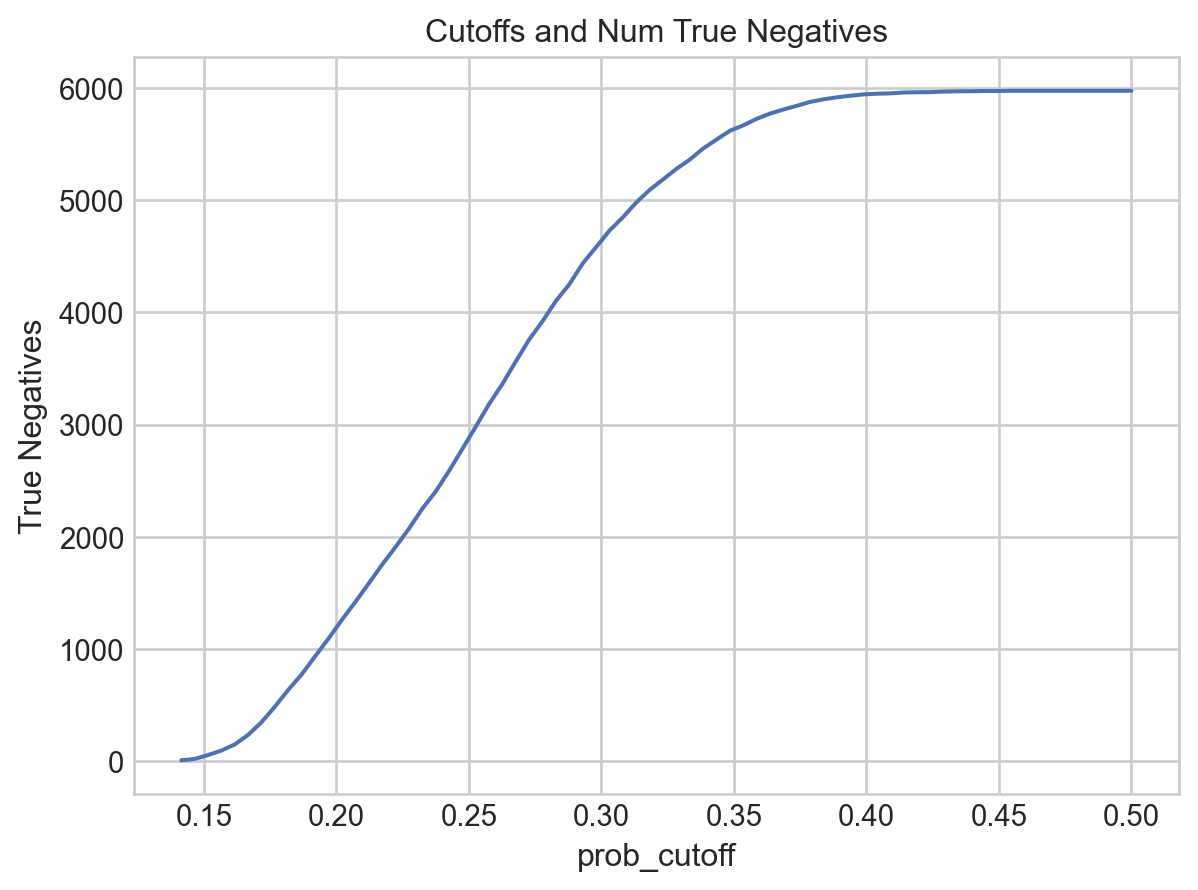
[25]:
(
    so.Plot(basic_gam, x="prob_cutoff", y="True Negatives")
    .add(so.Line())
    .label(title="Cutoffs and Num True Negatives")
    .theme({**style.library["seaborn-v0_8-whitegrid"]})
)
[25]:
[26]:
########
# Finally, query the optimal result from grid search
########

basic_gam_reasonable = basic_gam[basic_gam["True Negatives"] > 10]

min_reasonable = basic_gam_reasonable["False Omission Rate"].min()
good_at_min = basic_gam_reasonable.loc[
    basic_gam_reasonable["False Omission Rate"] == min_reasonable, "True Negatives"
].mean()
print(
    f"Best False Omission Rate is : {min_reasonable:.2%}.\n"
    f"At that you get {good_at_min:,.0f} True Negatives"
)
Best False Omission Rate is : 13.33%.
At that you get 91 True Negatives
Exercise 8
If the stakeholder wants to maximize true negatives and can tolerate a false omission rate of 19%, how many true negatives will they be able to enroll?
[27]:
# Here we see why doing this the rigorous, systematic way is so helpful.

most_true_negs = basic_gam.loc[
    basic_gam["False Omission Rate"] < 0.19, "True Negatives"
].max()

print(f"Most possible true negatives is: {most_true_negs:,.0f}")
Most possible true negatives is: 2,246
Let’s See This Interpretability!
We’re using GAMs for their interpretability, so let’s use it!
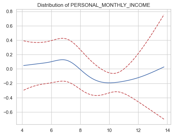
Exercise 9
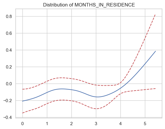
Plot the partial dependence plots for all your continuous factors with 95% confidence intervals (I have three, at this stage).
If you get an error like this when generating partial_dependence errors:
----> pdep, confi = gam.partial_dependence(term=i, X=XX, width=0.95)

...
ValueError: X data is out of domain for categorical feature 4. Expected data on [1.0, 2.0], but found data on [0.0, 0.0]
it’s because you have a variable set as a factor that doesn’t have values of 0. pyGAM is assuming 0 is the excluded category. Just recode the variable to ensure 0 is used to identify one of the categories.
[28]:
for i, term in enumerate(numeric_columns):
    print(i)
    print(term)
    XX = gam.generate_X_grid(term=i)
    pdep, confi = gam.partial_dependence(term=i, width=0.95)

    plt.figure()
    plt.plot(XX[:, i], pdep)
    plt.plot(XX[:, i], confi, c="r", ls="--")
    if i < len(numeric_columns):
        plt.title(f"Distribution of {numeric_columns[i]}")
    plt.show()
0
PERSONAL_MONTHLY_INCOME
1
AGE
2
MONTHS_IN_RESIDENCE
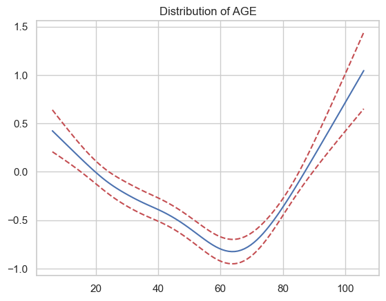
Exercise 10
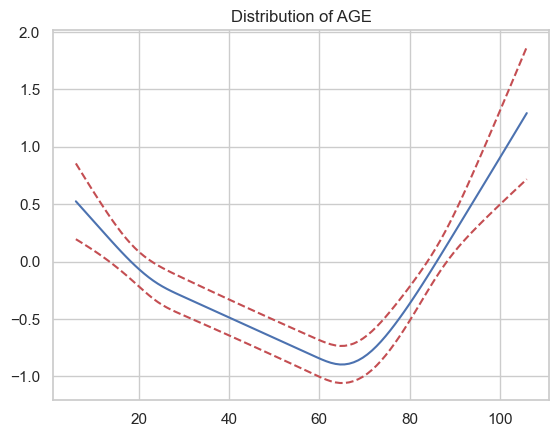
How does the partial correlation with respect to age look?
Seems like it’s an inverse-U relationship, but has some weird bumps in there. This probably isn’t the best example of why you’d want to impose functional form constraints, but it seems very unlikely that the wiggles between 20 and 60 represent real changes in risk — they’re just overfitting.
Arguably months in residence would be an even better choice for functional form constraints — no reason to think the relationship would go negative then positive between lot 2 and 4.
Exercise 11
Refit your model, but this time impose monotonicity or concavity/convexity on the relationship between age and credit risk (which makes more sense to you?). Fit the model and plot the new partial dependence.
[29]:
terms = (
    s(0)
    + s(1, constraints="convex")
    + s(2)
    + s(3)
    + f(4)
    + f(5)
    + f(6)
    + f(7)
    + f(8)
    + f(9)
)
gam_convex = LogisticGAM(terms=terms)
gam_convex.gridsearch(X_train.values, y_train.values)
0% (0 of 11) | | Elapsed Time: 0:00:00 ETA: --:--:--
  9% (1 of 11) |##                       | Elapsed Time: 0:00:01 ETA:   0:00:17
 18% (2 of 11) |####                     | Elapsed Time: 0:00:02 ETA:   0:00:13
 27% (3 of 11) |######                   | Elapsed Time: 0:00:03 ETA:   0:00:10
 36% (4 of 11) |#########                | Elapsed Time: 0:00:04 ETA:   0:00:08
 45% (5 of 11) |###########              | Elapsed Time: 0:00:05 ETA:   0:00:06
 54% (6 of 11) |#############            | Elapsed Time: 0:00:06 ETA:   0:00:05
 63% (7 of 11) |###############          | Elapsed Time: 0:00:07 ETA:   0:00:04
 72% (8 of 11) |##################       | Elapsed Time: 0:00:09 ETA:   0:00:03
 81% (9 of 11) |####################     | Elapsed Time: 0:00:11 ETA:   0:00:02
 90% (10 of 11) |#####################   | Elapsed Time: 0:00:13 ETA:   0:00:01
100% (11 of 11) |########################| Elapsed Time: 0:00:16 Time:  0:00:16
[29]:
LogisticGAM(callbacks=[Deviance(), Diffs(), Accuracy()],
   fit_intercept=True, max_iter=100,
   terms=s(0) + s(1) + s(2) + s(3) + f(4) + f(5) + f(6) + f(7) + f(8) + f(9) + intercept,
   tol=0.0001, verbose=False)
[30]:
i = 1
term = "AGE"
XX = gam_convex.generate_X_grid(term=i)
pdep, confi = gam_convex.partial_dependence(term=i, width=0.95)

plt.figure()
plt.plot(XX[:, i], pdep)
plt.plot(XX[:, i], confi, c="r", ls="--")
plt.title(f"Distribution of AGE")
plt.show()
Exercise 12
Functional form constraints are often about fairness or meeting regulatory requirements, but they can also prevent overfitting.
Does this change the number of “true negatives” you can enroll below a false omission rate of 19%?
[31]:
df_gam_convex = get_neg_stats(grid, gam_convex, X_test, y_test)

most_true_negs_convex = df_gam_convex.loc[
    df_gam_convex["False Omission Rate"] < 0.19, "True Negatives"
].max()

print(f"Most possible true negatives with convex age is: {most_true_negs_convex:,.0f}")
print(f"Compared to {most_true_negs:,.0f} true negatives when unconstrained.")
Most possible true negatives with convex age is: 2,130
Compared to 2,246 true negatives when unconstrained.
So… a little worse in terms of what you can squeeze out of things.
Exercise 13
In the preceding exercises, we allowed pyGAM to choose its own smoothing parameters / coefficient penalties. This makes life easy, but it isn’t always optimal, especially because when it does so, it picks the same smoothing penalty (the lambda in .summary()) for all terms.
(If you haven’t seen them let, penalities are designed to limit overfitting by, basically, “penalizing” big coefficients on different terms. This tends to push models towards smoother fits.)
To get around this, we can do a grid or random search. This is definitely a little slow, but let’s give it a try!
Then following the model given in the docs linked above, let’s do a random search. Make sure your initial random points has a shape of 100 x (the number of terms in your model).
[32]:
lams = np.random.rand(100, 10)
lams = lams * 6 - 3  # shift values to -3, 3
lams = 10**lams  # transforms values to 1e-3, 1e3

terms = (
    s(0)
    + s(1, constraints="convex")
    + s(2)
    + s(3)
    + f(4)
    + f(5)
    + f(6)
    + f(7)
    + f(8)
    + f(9)
)
gam_random_lam = LogisticGAM(terms=terms)
gam_random_lam.gridsearch(X_train.values, y_train.values, lam=lams)
  0% (0 of 100) |                        | Elapsed Time: 0:00:00 ETA:  --:--:--
  1% (1 of 100) |                        | Elapsed Time: 0:00:02 ETA:   0:03:53
  2% (2 of 100) |                        | Elapsed Time: 0:00:03 ETA:   0:03:12
  3% (3 of 100) |                        | Elapsed Time: 0:00:06 ETA:   0:03:24
  4% (4 of 100) |                        | Elapsed Time: 0:00:07 ETA:   0:03:06
  5% (5 of 100) |#                       | Elapsed Time: 0:00:08 ETA:   0:02:50
  6% (6 of 100) |#                       | Elapsed Time: 0:00:10 ETA:   0:02:37
  7% (7 of 100) |#                       | Elapsed Time: 0:00:11 ETA:   0:02:32
  8% (8 of 100) |#                       | Elapsed Time: 0:00:13 ETA:   0:02:31
  9% (9 of 100) |##                      | Elapsed Time: 0:00:14 ETA:   0:02:22
 10% (10 of 100) |##                     | Elapsed Time: 0:00:15 ETA:   0:02:15
 11% (11 of 100) |##                     | Elapsed Time: 0:00:16 ETA:   0:02:09
 12% (12 of 100) |##                     | Elapsed Time: 0:00:17 ETA:   0:02:04
 13% (13 of 100) |##                     | Elapsed Time: 0:00:18 ETA:   0:02:04
 14% (14 of 100) |###                    | Elapsed Time: 0:00:19 ETA:   0:02:00
 15% (15 of 100) |###                    | Elapsed Time: 0:00:20 ETA:   0:01:57
 16% (16 of 100) |###                    | Elapsed Time: 0:00:22 ETA:   0:01:57
 17% (17 of 100) |###                    | Elapsed Time: 0:00:23 ETA:   0:01:55
 18% (18 of 100) |####                   | Elapsed Time: 0:00:24 ETA:   0:01:51
 19% (19 of 100) |####                   | Elapsed Time: 0:00:25 ETA:   0:01:49
 20% (20 of 100) |####                   | Elapsed Time: 0:00:27 ETA:   0:01:49
 21% (21 of 100) |####                   | Elapsed Time: 0:00:28 ETA:   0:01:46
 22% (22 of 100) |#####                  | Elapsed Time: 0:00:29 ETA:   0:01:43
 23% (23 of 100) |#####                  | Elapsed Time: 0:00:30 ETA:   0:01:41
 24% (24 of 100) |#####                  | Elapsed Time: 0:00:32 ETA:   0:01:41
 25% (25 of 100) |#####                  | Elapsed Time: 0:00:33 ETA:   0:01:39
 26% (26 of 100) |#####                  | Elapsed Time: 0:00:34 ETA:   0:01:37
 27% (27 of 100) |######                 | Elapsed Time: 0:00:35 ETA:   0:01:35
 28% (28 of 100) |######                 | Elapsed Time: 0:00:36 ETA:   0:01:34
 29% (29 of 100) |######                 | Elapsed Time: 0:00:37 ETA:   0:01:32
 30% (30 of 100) |######                 | Elapsed Time: 0:00:39 ETA:   0:01:32
 31% (31 of 100) |#######                | Elapsed Time: 0:00:41 ETA:   0:01:32
 32% (32 of 100) |#######                | Elapsed Time: 0:00:42 ETA:   0:01:30
 33% (33 of 100) |#######                | Elapsed Time: 0:00:44 ETA:   0:01:29
 34% (34 of 100) |#######                | Elapsed Time: 0:00:46 ETA:   0:01:29
 35% (35 of 100) |########               | Elapsed Time: 0:00:47 ETA:   0:01:27
 36% (36 of 100) |########               | Elapsed Time: 0:00:48 ETA:   0:01:26
 37% (37 of 100) |########               | Elapsed Time: 0:00:50 ETA:   0:01:25
 38% (38 of 100) |########               | Elapsed Time: 0:00:51 ETA:   0:01:23
 39% (39 of 100) |########               | Elapsed Time: 0:00:52 ETA:   0:01:21
 40% (40 of 100) |#########              | Elapsed Time: 0:00:53 ETA:   0:01:20
 41% (41 of 100) |#########              | Elapsed Time: 0:00:54 ETA:   0:01:19
 42% (42 of 100) |#########              | Elapsed Time: 0:00:55 ETA:   0:01:17
 43% (43 of 100) |#########              | Elapsed Time: 0:00:57 ETA:   0:01:15
 44% (44 of 100) |##########             | Elapsed Time: 0:00:58 ETA:   0:01:14
 45% (45 of 100) |##########             | Elapsed Time: 0:00:59 ETA:   0:01:12
 46% (46 of 100) |##########             | Elapsed Time: 0:01:00 ETA:   0:01:10
 47% (47 of 100) |##########             | Elapsed Time: 0:01:01 ETA:   0:01:09
 48% (48 of 100) |###########            | Elapsed Time: 0:01:02 ETA:   0:01:07
 49% (49 of 100) |###########            | Elapsed Time: 0:01:04 ETA:   0:01:07
 50% (50 of 100) |###########            | Elapsed Time: 0:01:05 ETA:   0:01:05
 51% (51 of 100) |###########            | Elapsed Time: 0:01:06 ETA:   0:01:04
 52% (52 of 100) |###########            | Elapsed Time: 0:01:07 ETA:   0:01:02
 53% (53 of 100) |############           | Elapsed Time: 0:01:09 ETA:   0:01:01
 54% (54 of 100) |############           | Elapsed Time: 0:01:10 ETA:   0:00:59
 55% (55 of 100) |############           | Elapsed Time: 0:01:10 ETA:   0:00:58
 56% (56 of 100) |############           | Elapsed Time: 0:01:12 ETA:   0:00:57
 57% (57 of 100) |#############          | Elapsed Time: 0:01:13 ETA:   0:00:55
 58% (58 of 100) |#############          | Elapsed Time: 0:01:15 ETA:   0:00:54
 59% (59 of 100) |#############          | Elapsed Time: 0:01:16 ETA:   0:00:52
 60% (60 of 100) |#############          | Elapsed Time: 0:01:16 ETA:   0:00:51
 61% (61 of 100) |##############         | Elapsed Time: 0:01:18 ETA:   0:00:50
 62% (62 of 100) |##############         | Elapsed Time: 0:01:19 ETA:   0:00:48
 63% (63 of 100) |##############         | Elapsed Time: 0:01:20 ETA:   0:00:47
 64% (64 of 100) |##############         | Elapsed Time: 0:01:21 ETA:   0:00:45
 65% (65 of 100) |##############         | Elapsed Time: 0:01:23 ETA:   0:00:44
 66% (66 of 100) |###############        | Elapsed Time: 0:01:24 ETA:   0:00:43
 67% (67 of 100) |###############        | Elapsed Time: 0:01:25 ETA:   0:00:42
 68% (68 of 100) |###############        | Elapsed Time: 0:01:26 ETA:   0:00:40
 69% (69 of 100) |###############        | Elapsed Time: 0:01:27 ETA:   0:00:39
 70% (70 of 100) |################       | Elapsed Time: 0:01:29 ETA:   0:00:38
 71% (71 of 100) |################       | Elapsed Time: 0:01:30 ETA:   0:00:36
 72% (72 of 100) |################       | Elapsed Time: 0:01:31 ETA:   0:00:35
 73% (73 of 100) |################       | Elapsed Time: 0:01:33 ETA:   0:00:34
 74% (74 of 100) |#################      | Elapsed Time: 0:01:34 ETA:   0:00:33
 75% (75 of 100) |#################      | Elapsed Time: 0:01:36 ETA:   0:00:32
 76% (76 of 100) |#################      | Elapsed Time: 0:01:36 ETA:   0:00:30
 77% (77 of 100) |#################      | Elapsed Time: 0:01:38 ETA:   0:00:29
 78% (78 of 100) |#################      | Elapsed Time: 0:01:39 ETA:   0:00:28
 79% (79 of 100) |##################     | Elapsed Time: 0:01:40 ETA:   0:00:26
 80% (80 of 100) |##################     | Elapsed Time: 0:01:42 ETA:   0:00:25
 81% (81 of 100) |##################     | Elapsed Time: 0:01:43 ETA:   0:00:24
 82% (82 of 100) |##################     | Elapsed Time: 0:01:44 ETA:   0:00:22
 83% (83 of 100) |###################    | Elapsed Time: 0:01:46 ETA:   0:00:21
 84% (84 of 100) |###################    | Elapsed Time: 0:01:47 ETA:   0:00:20
 85% (85 of 100) |###################    | Elapsed Time: 0:01:48 ETA:   0:00:19
 86% (86 of 100) |###################    | Elapsed Time: 0:01:50 ETA:   0:00:17
 87% (87 of 100) |####################   | Elapsed Time: 0:01:51 ETA:   0:00:16
 88% (88 of 100) |####################   | Elapsed Time: 0:01:53 ETA:   0:00:15
 89% (89 of 100) |####################   | Elapsed Time: 0:01:54 ETA:   0:00:14
 90% (90 of 100) |####################   | Elapsed Time: 0:01:55 ETA:   0:00:12
 91% (91 of 100) |####################   | Elapsed Time: 0:01:56 ETA:   0:00:11
 92% (92 of 100) |#####################  | Elapsed Time: 0:01:58 ETA:   0:00:10
 93% (93 of 100) |#####################  | Elapsed Time: 0:01:59 ETA:   0:00:08
 94% (94 of 100) |#####################  | Elapsed Time: 0:02:00 ETA:   0:00:07
 95% (95 of 100) |#####################  | Elapsed Time: 0:02:01 ETA:   0:00:06
 96% (96 of 100) |###################### | Elapsed Time: 0:02:03 ETA:   0:00:05
 97% (97 of 100) |###################### | Elapsed Time: 0:02:04 ETA:   0:00:03
 98% (98 of 100) |###################### | Elapsed Time: 0:02:05 ETA:   0:00:02
 99% (99 of 100) |###################### | Elapsed Time: 0:02:07 ETA:   0:00:01
100% (100 of 100) |######################| Elapsed Time: 0:02:08 Time:  0:02:08
[32]:
LogisticGAM(callbacks=[Deviance(), Diffs(), Accuracy()],
   fit_intercept=True, max_iter=100,
   terms=s(0) + s(1) + s(2) + s(3) + f(4) + f(5) + f(6) + f(7) + f(8) + f(9) + intercept,
   tol=0.0001, verbose=False)
Exercise 14
How many true negatives can you get now at a less than 19% False Omission Rate?
[33]:
df_gam_random_lam = get_neg_stats(grid, gam_random_lam, X_test, y_test)

most_true_negs_lam = df_gam_random_lam.loc[
    df_gam_random_lam["False Omission Rate"] < 0.19, "True Negatives"
].max()

print(
    f"Most possible true negatives with grid search of regularization weights is: {most_true_negs_lam:,.0f}"
)
print(f"Compared to {most_true_negs:,.0f} true negatives when unconstrained.")
Most possible true negatives with grid search of regularization weights is: 2,307
Compared to 2,246 true negatives when unconstrained.
Exercise 15
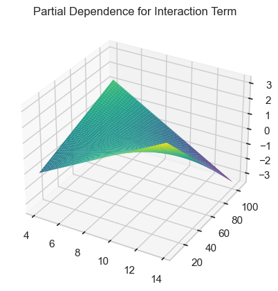
Add an interaction term between age and personal income.
[34]:
from pygam import te

terms = (
    s(0)
    + s(1, constraints="convex")
    + s(2)
    + s(3)
    + f(4)
    + f(5)
    + f(6)
    + f(7)
    + f(8)
    + f(9)
    + te(0, 1)
)
gam_interact = LogisticGAM(terms=terms)
gam_interact.gridsearch(X_train.values, y_train.values)
  0% (0 of 11) |                         | Elapsed Time: 0:00:00 ETA:  --:--:--
  9% (1 of 11) |##                       | Elapsed Time: 0:00:05 ETA:   0:00:59
 18% (2 of 11) |####                     | Elapsed Time: 0:00:10 ETA:   0:00:45
 27% (3 of 11) |######                   | Elapsed Time: 0:00:14 ETA:   0:00:38
 36% (4 of 11) |#########                | Elapsed Time: 0:00:18 ETA:   0:00:31
 45% (5 of 11) |###########              | Elapsed Time: 0:00:21 ETA:   0:00:25
 54% (6 of 11) |#############            | Elapsed Time: 0:00:25 ETA:   0:00:20
 63% (7 of 11) |###############          | Elapsed Time: 0:00:28 ETA:   0:00:16
 72% (8 of 11) |##################       | Elapsed Time: 0:00:31 ETA:   0:00:11
 81% (9 of 11) |####################     | Elapsed Time: 0:00:34 ETA:   0:00:07
 90% (10 of 11) |#####################   | Elapsed Time: 0:00:40 ETA:   0:00:04
100% (11 of 11) |########################| Elapsed Time: 0:00:42 Time:  0:00:42
[34]:
LogisticGAM(callbacks=[Deviance(), Diffs(), Accuracy()],
   fit_intercept=True, max_iter=100,
   terms=s(0) + s(1) + s(2) + s(3) + f(4) + f(5) + f(6) + f(7) + f(8) + f(9) + te(0, 1) + intercept,
   tol=0.0001, verbose=False)
Exercise 16
Now visualize the partial dependence interaction term.
[35]:
import matplotlib.pyplot as plt
from mpl_toolkits import mplot3d
[36]:
XX = gam_interact.generate_X_grid(term=10, meshgrid=True)
Z = gam_interact.partial_dependence(term=10, X=XX, meshgrid=True)
[37]:
ax = plt.axes(projection="3d")
Z = Z.reshape(XX[0].shape)
ax.plot_surface(XX[0], XX[1], Z, cmap="viridis", edgecolor="none")
ax.set_title("Partial Dependence for Interaction Term")
plt.show()
Exercise 17
Finally, another popular interpretable model is the ExplainableBoostingClassifier. You can learn more about it here, though how much sense it will make to you may be limited if you aren’t familiar with gradient boosting yet. Still, at least one of your classmates prefers it to pyGAM, so give it a try using this code:
from interpret.glassbox import ExplainableBoostingClassifier
from interpret import show
import warnings

ebm = ExplainableBoostingClassifier()
ebm.fit(X_train, y_train)

with warnings.catch_warnings():
   warnings.simplefilter("ignore")

   ebm_global = ebm.explain_global()
   show(ebm_global)

   ebm_local = ebm.explain_local(X_train, y_train)
   show(ebm_local)
[38]:
from interpret.glassbox import ExplainableBoostingClassifier
from interpret import show
import warnings

ebm = ExplainableBoostingClassifier()
ebm.fit(X_train, y_train)

with warnings.catch_warnings():
    warnings.simplefilter("ignore")

    ebm_global = ebm.explain_global()
    show(ebm_global)

    ebm_local = ebm.explain_local(X_train, y_train)
    show(ebm_local)